|
In my previous
article entitled "The Sunday Scientist," I described
my trials and tribulations with the first lab assignment in
Dr. Ron's online sand bed ecology class. It should come as
no surprise that the other lab assignments were equally challenging.
I know that for both students and instructor alike, this class
required a substantial investment of time and effort. I, for
one, feel the time was well spent and the effort worthwhile.
So little has been done to quantify the processes occurring
in captive marine environments that any contribution to this
knowledge base has value. I would like to encourage my fellow
reefkeepers, especially the experienced aquarists, to repeat
our experiments in their own tanks. The larger the sample
size, the more conclusions we can draw from the data. No matter
how long you've kept a reef tank, the results of some of the
tests may surprise you, and the wonder of discovery is a reward
unto itself.
While our first class assignment was to
define the physical parameters of our sand bed by determining
the grain size distribution, (this is the infamous "Sand
Castles 1A" you always heard they offered in college),
the second lab assignment was designed to determine the environment's
chemical parameters. The plan was to use a syringe with a
fine needle to extract water from the sand bed, and test that
water for ammonia, nitrite, nitrate, phosphate, pH, dissolved
oxygen, sulfide and copper. Samples were to be collected from
the overlying water, and then at two-centimeter increments
down to the bottom of the bed. Since my sand bed's depth averages
ten centimeters, I needed six water samples for each test.
Each chemical was to be measured in three different places
in the sand bed. Eight chemicals, six samples and three replicants
worked out to 144 water samples ranging from three to ten
milliliters. (Thank goodness I didn't go with a six-inch sand
bed!) While the sheer number of samples seemed daunting, using
a syringe and needle to extract water from the sand bed didn't
sound like it would be that big a deal. (If only I had a dime
for every time I've thought THAT since I've been in the hobby!)
I acquired a selection of syringes and needles from a pharmacist
friend and went to work.
It Ain't Easy
After my dismal failure at one-handed sand
coring from my first lab assignment, I decided to practice
the needle and syringe method of water extraction first in
the refugium, where I was free to use both hands. Once again,
I was confounded by the really fine sand in my system. While
it makes a great sand bed, it was impossible to suck water
through it with a needle. With smaller needles, I couldn't
pull hard enough on the large syringe to get the water to
flow in. Larger gauge needles clogged with sand. Even if I
had been able to find a syringe and needle combination that
would work, I still would have had to snorkel in the tank
to get both hands to the sand bed. (And, yes, for those men
in the audience, I did ask my husband to give the syringe
a try. While he can easily open any jar for me, he couldn't
get water into the syringe either).
I learned the lesson, "If at first
you don't succeed, use a bigger tool" from watching my
dad work in the garage when I was a kid. So, my husband and
I came up with the brilliant plan to use a hand pump, like
the one used to bleed brakes on motorcycles, to create enough
suction to get the water into the syringe. A couple of hours
of work with rigid airline tubing, air hose, pieces of syringes,
and assorted necessities such as tape and superglue, yielded
a device capable of exerting 45 pounds/square inch of suction
on a piece of rigid airline tubing with a needle attached.
While it was truly an impressive device (of which MacGyver
would have been proud), it was nonetheless utterly useless.
Once again, I found myself sitting at the kitchen table with
my head in my hands. (Just in case you were curious, the way
the real scientists do it is by taking core samples, flash
freezing them, cutting them into pieces and then extracting
the water with a centrifuge. But, alas, after purchasing all
the test kits for class there was no money left in my science
budget for such things, so a less expensive solution had to
be found.)
A suggestion from a friend helped lead
me to the ultimate solution to the problem. I ended up using
a siphon made from the smallest diameter rigid airline tubing
I could find. I made marks on it every two centimeters and
stuffed a wad of cotton into the end of the tubing. I attached
an air hose to the opposite end of the tube.
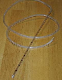
My high-tech water collection device. The cotton stuffed
into the end of the tube slowed the flow of water and
kept sand out of the sample. |
By pushing the rigid airline into the sand
to whatever depth I needed, I used the natural siphon effect
to draw water slowly into the tube. The wad of cotton helped
slow the flow of water and keep sand out of the tube. I used
the air hose like a straw to apply suction when needed, or
provide backpressure if the water was entering the tubing
too quickly. It was important to collect the water samples
as slowly as possible. If they collected too quickly, I would
have been collecting water from levels above or below my target
level. Each milliliter took two minutes to collect. My rough
calculations say that I extracted approximately 600 milliliters
of water at two minutes per milliliter for a grand total of
20 hours. I spent another five hours actually performing the
tests.
The tests themselves were a challenge,
as any of you who has tried reading colormetric tests knows.
I carried my trays of test tubes from room to room, from lights
to windows trying to discern ever-so-slight differences in
shades of pink, blue and yellow. If it sounds to you like
this process was less than exact, you are absolutely right.
(Fortunately for me, analyzing the data and compensating for
errors were Dr. Ron's problems!) In all, I know it took me
a good two weeks to complete the chemical analysis.
 |
I found it easiest to first collect all the water samples
for each test, then perform the test.
|
|
Ammonia
|
|
Sulfide
|
|
NO3
|
|
|
|
|
|
|
|
|
|
|
|
|
|
|
|
|
Depth(cm)
|
Rep
1
|
Rep
2
|
Rep
3
|
|
Depth(cm)
|
Rep
1
|
Rep
2
|
Rep
3
|
|
Depth(cm)
|
Rep
1
|
Rep
2
|
Rep
3
|
|
0
|
0
|
0
|
0
|
|
0
|
0
|
0
|
0
|
|
0
|
2
|
2
|
2
|
|
2
|
0
|
0
|
0
|
|
2
|
0
|
0
|
0
|
|
2
|
25
|
15
|
20
|
|
4
|
0
|
0
|
0
|
|
4
|
0
|
0
|
0
|
|
4
|
15
|
10
|
5
|
|
6
|
0
|
0
|
0
|
|
6
|
0
|
0
|
0
|
|
6
|
10
|
20
|
10
|
|
8
|
0
|
0
|
0.2
|
|
8
|
0
|
0
|
0
|
|
8
|
2
|
15
|
10
|
|
10
|
0.5
|
0.2
|
0.5
|
|
10
|
0
|
0
|
0
|
|
10
|
1
|
2
|
10
|
|
|
|
|
|
|
|
|
|
|
|
|
|
|
|
|
pH |
|
Oxygen |
|
NO2 |
|
|
|
|
|
|
|
|
|
|
|
|
|
|
|
|
Depth(cm)
|
Rep
1
|
Rep
2
|
Rep
3
|
|
Depth(cm)
|
Rep
1
|
Rep
2
|
Rep
3
|
|
Depth(cm)
|
Rep
1
|
Rep
2
|
Rep
3
|
|
0
|
7.7
|
7.7
|
7.7
|
|
0
|
7
|
7
|
7
|
|
0
|
0.01
|
0
|
0
|
|
2
|
8
|
7.6
|
7.7
|
|
2
|
6
|
6
|
6
|
|
2
|
0.1
|
0.01
|
0.01
|
|
4
|
7.7
|
7.6
|
7.7
|
|
4
|
6
|
6
|
7
|
|
4
|
0.1
|
0.025
|
0.01
|
|
6
|
7.5
|
7.6
|
7.5
|
|
6
|
6
|
5
|
7
|
|
6
|
0.01
|
0.025
|
0.015
|
|
8
|
7.5
|
7.5
|
7.5
|
|
8
|
5
|
6
|
6
|
|
8
|
0.01
|
0.025
|
0.05
|
|
10
|
7.4
|
7.4
|
7.5
|
|
10
|
5
|
6
|
5
|
|
10
|
0.01
|
0.2
|
0.2
|
Phosphate and copper were undetectable at all depths.
The chemical analysis of my sand bed yielded
a couple of interesting results. First, conventional wisdom
held that the lower level of my sand bed would be an anaerobic
zone. However, my tests showed a value of 5ppm dissolved oxygen
at the very bottom of the bed, a depth of 10 cm. Second, I
found only small, isolated patches of hydrogen sulfide that
tended to be relatively close to the sand bed's surface. I
had expected to find a layer of anoxic sediments with hydrogen
sulfide at the bottom of my sand bed. I was pleased to learn
that the ammonia, nitrite and nitrate levels indicated that
my sand bed was functioning as expected with regard to the
nitrogen cycle. In fact, it seems to work just like the aquarium
books say it does; imagine that!
The Fun Stuff
Finally! With the mechanical and chemical
stuff out of the way, we could get down to the business of
counting animals. For the first week, we conducted a microscopic
safari. Several of my classmates had not attended Dr. Ron's
class in invertebrate zoology, so they didn't really know
how to identify the animals we were going to be counting.
We all needed to agree on our identification of the animals
if our counts were to be compared; hence, the safari. I used
a plastic bulb-tipped pipette to extract small quantities
of sand from my tank and searched for critters. The idea was
to compile a photographic catalog of the animals with at least
a genus-level identification. The result was the geekiest
scavenger hunt ever, with everyone submitting photos of worms,
pods, mollusks and even mites. Dr. Ron provided several animal
identification keys so we could put a name on all of the animals
we found.
 |
|
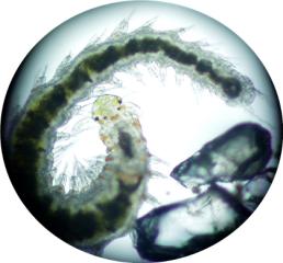 |
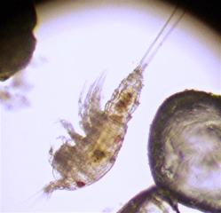
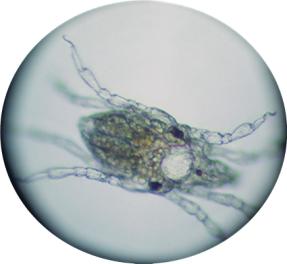
Copepods (left) and polychaete worms (right)
were two of the most common animals I found in my sand
bed.
Many folks, however, have never had a chance to get a close
look at these fascinating little critters.
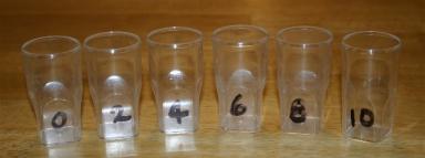
With an identification guide to work with,
the real work started. In order to estimate the population
of the various species of animals living in my substrate,
I had to collect and count the animals in a defined area.
The first sample I used was a one-inch diameter circle. To
get the proper sample area, I cut a piece of clear tubing
from a package of underwater epoxy, placed it into the sand
about an inch deep, then carefully siphoned the top one centimeter
of sand from within the tube into a glass beaker. I used an
eyedropper to transfer small amounts of sand and water into
a Petri dish. Only one layer of sand grains could be put into
the Petri dish at a time, otherwise animals would be obscured
by the substrate. (I had twelve Petri dishes to count in my
first sample.)
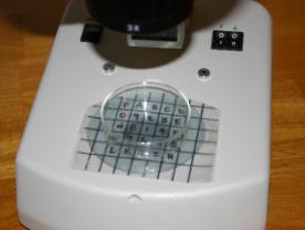
I had made a one-centimeter grid on a square
of clear plastic and had numbered each square. The Petri dish
was placed on top of the grid on the lighted stage of my dissecting
microscope.
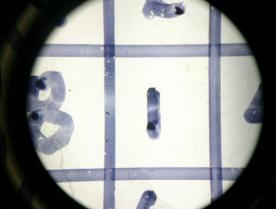
Using thirty times magnification, I examined
each grid square and tallied the animals. My first sample
took three and a half hours to count. I found three hundred
larger animals including nematodes, copepods, ostracodes and
segmented worms. I counted at least five hundred large ciliates.
I had to ignore the small ciliates and sessile animals such
as forams or I could have been counting all day!
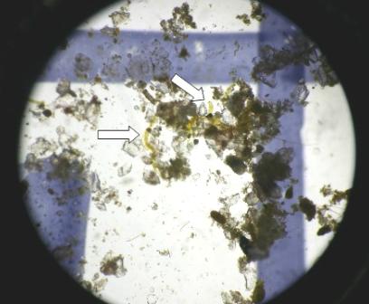
This photograph shows the upper quadrant of one grid square
with
arrows pointing to several worms.
One of the major challenges of counting
the animals was their stubborn refusal to stay in one square.
Copepods were the worst! They bounced around the Petri dish
like fleas on a hot plate. I had to keep switching between
the ten-times and thirty-times magnification to try to ensure
I hadn't counted any copepods twice. I'm sure my conservatism
meant I ended up underestimating the number of copepods in
my samples. (Blame it on too many years as an accountant).
The lab assignment called for a total
of five counts. In addition to my main tank, I had done some
of the prior lab work on my refugium, so I wanted to include
a couple of counts from it for comparison. Taking six more
samples at three and a half hours each was a little more than
my schedule would allow, so I reduced my sample diameter from
25.4mm (1 inch) to 15mm. Even with the smaller sample size,
I was still finding an average of 156 larger animals and it
took about two and a half hours to get through each count.
In our reading assignments for class, we discovered that in
real field surveys of benthic communities, the sample sizes
were one square meter. (Of course, the folks doing such a
survey would not have tried counting the animals alive.) Fortunately
for my animals, most were returned unscathed to their homes.
I must confess, however, a few unfortunate individuals did
not survive my clumsy attempts to pin them under a cover slip
so I could take their picture. (And you thought it was hard
to get a two-year old to hold still for a family portrait!)
Here are a few of the most interesting
animals I found in my sand bed.
 |
|
 |
|
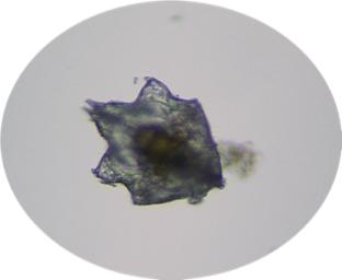
This mite is a relative of the spider.
|
|
|
 |
|
|
|
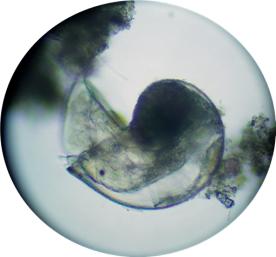
Here we have a newly settled snail.
|
|
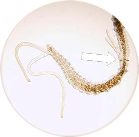
This worm is budding off another worm. The arrow shows
the point where a new head and palps are forming.
|
For those curious types, these pictures
were taken through my Olympus BH-2 microscope with an Olympus
E-10 digital camera. I found the animals with the dissecting
scope, then used an eyedropper to transfer them to a depression
slide. Most of these pictures were done at between 100X -
400X magnification.
The results of the counts from my display
tank are as follows:
| Animal |
Count
1 (25.4mm) |
Count
2 (15mm) |
Count
3 (15mm) |
Count
4 (15mm) |
Count
5 (15mm) |
|
Nematode
|
91
|
62
|
43
|
71
|
90
|
|
Ostracode
|
25
|
13
|
20
|
11
|
17
|
|
Copepod
|
131
|
71
|
23
|
53
|
22
|
|
Syllidae
|
1
|
0
|
1
|
1
|
0
|
|
Dorvilleidae
|
3
|
0
|
0
|
6
|
0
|
|
Cirratulid
|
46
|
27
|
19
|
44
|
2
|
|
Ctenodrillid
|
1
|
0
|
0
|
0
|
0
|
|
Magelonidae
|
3
|
6
|
0
|
0
|
0
|
|
mite/flatworm
|
0
|
0
|
1
|
0
|
20
|
|
|
301
|
179
|
107
|
186
|
151
|
After averaging the samples and converting
the area, my average density was 919,922 animals per square
meter (excluding ciliates). I was impressed!
What Does It All Mean?
I know that many of you are curious to
know what conclusions (if any) can be drawn from the data
collected in our class. There are those of you who will ask,
"What possible conclusions can be reached with such a
small and imprecise set of data?" I wondered that myself,
and, like you, will have to wait to see what Dr. Ron can make
of it. I do believe, however, that if we had data from one
hundred tanks, instead of just ten, the data would be much
more useful. So, how about it… are you game?
|