|
Introduction
One of the most
vexing concerns of reef aquarists is the problem of water
chemistry. These concerns are founded in the knowledge that
reef aquaria are really very tiny analogues of natural systems,
and because of their small size chemical changes could occur
that could adversely impact their livestock. The composition
of natural sea water (NSW) is taken as the basis for measuring
all changes in the water in aquaria, even though the standard
for such natural seawater has historically been from the North
Sea and not coral reefs. Chemical concentrations of most materials
in seawater are presumed by most aquarists to be "conservative"
and unchangeable, consequently, it is presumed that any changes
away from the NSW concentrations are detrimental. On the gross
scale of the world ocean's such a supposition has some validity,
however in the close environment of the reef significant changes
in many chemical constituents can and do occur. However, the
data detailing with changes in coral reef water chemistry
are sparse, and difficult to relate to the standard reef aquarium.
Most aquarists, probably correctly, feel that they can't go
wrong if they pursue a course of aquarium water chemistry
management based trying to maintain "natural levels."
Implicit in such
a management plan, although seldom directly stated, is the
feeling that organisms somehow "use up," "change,"
or "consume" many of these chemicals, and in doing
so, forever remove the chemicals from that reef aquarium system.
This assumption is not completely false, some chemicals are
"used up" and removed from the system, but most
are not. Organisms are dynamic entities, and while some chemicals
are temporarily sequestered away, such chemicals generally
remain available in the system due to metabolic turnover.
The only real exceptions to this as far as organisms are concerned
are those chemicals, such as calcium, which get incorporated
into an insoluble matrix. Once the chemical is removed from
solution, even if that matrix, such as a coral skeleton or
clam shell, remains in the aquarium, it is beyond the use
of most organisms.
Another more important
variable of these systems is chemical export via some sort
of filtration or organism removal. The various types of filtration
are widely regarded as very efficient, not at all efficient,
or useless, depending on the authority consulted and presumably
the whim of the moment. Unfortunately, there are few hard
data to support any of the suppositions about export, except
that it occurs. I hope to address the question of export methodologies
and their effectiveness in a future research project, but
for the present, we simply don’t have a good handle on
what, or how, various chemicals leave our aquaria.
If we just started
with sea water and had to deal with its changes over time,
that would make the determination of what is happening in
our systems relatively easy. Note that I didn't say, "Easy"
but "relatively easy." However, we don't generally
start with real seawater. Relatively few aquarists have access
to natural seawater, and must use dried artificial mixes and
some type of water to make the medium they put into their
aquaria. These mixtures may vary significantly in many regards
from natural water (See Atkinson and Bingman, 1999: AFM-online).
Additionally, and importantly, we continually further alter
the chemical constituents of our systems by adding food, and
various other additives. The food is added based on our observations
and knowledge of the organisms' needs. The other additives
are added based on chemical tests, belief in the advertisements
of the additive producers, barometric pressure, a toss of
the dice, or maybe, just maybe, some rational guesstimate
of depletion rates.
This report is
the first of several, at least three and maybe more, examining
the chemical constituents of marine aquarium water. It is
a follow-up to my "Food and Additive Study" done
about two years ago. In that project, I examined the chemical
constituency of 15 popular foods and additives used by aquarists.
The data from that study are available here: AFM-online.
Using those data, we can reasonably well determine what chemicals
may enter our systems. However, until now, we really didn't
have any really good idea of what exactly is in our systems.
This study is an
attempt to describe the chemical constituents of an "Average
Reef Tank." The goal was to survey as wide a database
as possible in the hope that the results of the study would
be representative of reef tanks, in general. To that end,
I advertised for volunteers willing to pay for the analysis
of their tank water. I had hoped to get at least 15 volunteers,
I got 18, and we were able to analyze the data from 23 different
systems as well as one sample of artificial sea water. The
participants had to answer a somewhat detailed questionnaire
about their systems, and how those systems were maintained.
Those responses and further analyses will constitute the basis
for the forthcoming articles. This article will deal with
the basic results of the water analyses of these systems.

Materials and Methods
I am an invertebrate
zoologist, not an analytical chemist, so I couldn't do the
necessary tests. They were done by a commercial analytical
laboratory in the Seattle region.
The laboratory
was:
AM TEST LABORATORIES,
INC.
14603 NE 87th Street
Redmond, WA 98052.
They used two basic
sources for analytical techniques:
EPA = Methods for
Chemical Analysis of Water and Wastes, 1983 (available from
National Technical Information Service, 5285 Port Royal Road,
Springfield, VA 22161, Stock No. NTIS PB84-128677);
SM = American Public
Health Association. 1992. Standard Methods for the examination
of water and wastewater, 18th ed. American Public Health Association,
Washington, D.C.
The concentrations
were determined by Inductively Coupled Plasma Emission Spectrometry
or ICP Scan, EPA method 200.7.
| • |
The concentrations
of the following metals or ions in the unaltered product
were determined: Aluminum, Antimony, Arsenic, Barium,
Beryllium, Boron, Cadmium, Calcium, Chromium, Cobalt,
Copper, Iodide, Iron, Lead, Lithium, Magnesium, Manganese,
Mercury, Molybdenum, Nickel, Phosphorus, Potassium, Selenium,
Silicon, Silver, Sodium, Strontium, Sulfur, Thallium,
Tin, Titanium, Vanadium, Yttrium, and Zinc. |
| • |
Ammonia Nitrogen,
Total Kjeldahl Nitrogen, Nitrate and Nitrite Nitrogen
were also determined using these methods: EPA 350.1; EPA
351.3; and EPA 353.2, respectively. |
| • |
Additionally the
samples were analyzed using the methods indicated to determine
the percentages of Moisture, EPA 160.3; Carbohydrates,
AOAC pg 922; Fat, AOAC 30.049 11th edition, 1970; and
Total Protein, SM 4500-N. The percent of the dissolved
solids present as Ash was also determined using EPA 160.4
and the number of Calories per gram of the sample was
also determined by ASTM D240. |
After verification
of the participants, the laboratory was contacted and they
sent sampling materials to me, these were plastic bottles
labeled for each of three necessary samples from each aquarium.
In total, each sample consisted of three 500 ml samples of
aquarium water, one each for the metals, nitrogen chemistry,
and conventional nutrients. After I received the sampling
bottles, I prepackaged them and distributed them to the participants
along with a questionnaire and instructions. The samples were
returned me and then sent to the analytical laboratory. After
the analysis, the data were returned to me, and electronically
coded for analysis.
There were 24 samples
analyzed: 23 aquarium samples, and one sample, of Instant
Ocean(tm) (IO), prepared with 0 total dissolved solids RO/DI,
mixed to 35 ppt, and stored for two weeks prior to testing
in an FDA food-grade container. For comparative analyses,
the chemical constituents for NSW were obtained from Weast,
1966.
The samples constituted
independent samples without replication. The lack of replication
significantly reduces the options for statistical analyses,
however, it was necessary to obtain as wide a sample as possible.
Given the cost of the sample analysis, analysis of replicates
was simply too expensive. The lack of sample replicates precluded
the use of tests such as analyses of variance (ANOVA), and
other tests on means and variances.
However, basic
descriptive techniques were possible as were many sample-to-sample
comparisons. These analyses were dependent on the numerical
values of the concentrations of the various constituents.
The numerical values ranged from values as small as 0.0001
µg/l to as high as 12000 µg/l. This is a range
variation in abundance of 100,000,000 times. Obviously, in
any comparison those samples with high numerical values of
any chemical could overwhelm the information in those with
smaller amounts of chemicals. Consequently, all tests were
run twice, once using untransformed data, and the second time
with a log normal transformation of the data. A log normal
transformation of the data involves taking the value for the
datum, adding one to it, and taking the natural logarithm
of the sample. Algebraically, this transformation is indicated
by the following terminology: ln(x+1), where x = the sample
datum. Such a log-normal transformation is commonly done in
those analyses where data may very over several orders of
magnitude and it reduces the influence of large values and
increases the influence of smaller values. The transformation
has known properties and quite useful in comparisons involving
widely dissimilar data values. In these samples, this transformation
reduced the influence of relatively highly concentrated materials,
for example Sodium, Sulfur, and Magnesium.
In the initial
analyses, the salinity varied widely. I presumed many of the
constituent abundances were correlated with salinity; for
example, if two batches artificial salt mix was made up, one
a concentration of 30 ppt, and the other to a concentration
36 ppt, there would be differences in all of the materials
found in the two samples. However, none of these differences
would be due to any "in tank" changes or variables.
Consequently I normalized all data by adjusting all the samples
to the same sodium concentration as found in the tabled value
for NSW; this was done by multiplying all concentrations by
a constant consisting of the sodium concentration divided
by the sodium concentration in NSW. Finally, after the initial
analyses were completed, I removed from consideration all
chemicals found in NSW but below detection limits in all of
the samples.
The elements removed
from these analyses were: Beryllium, Cadmium, Chromium, Iron,
Lead, Manganese, Mercury, Selenium, Silver and Yttrium.
Descriptive statistics
were determined on a spreadsheet, Quattro Pro (Corel, 1997).
The relationships between and within the samples were investigated
using a series of analytical programs called the Community
Analyses System, V. 5.0 (Bloom, 1994). Initially, the samples
underwent a process called classification. The index used
to classify the samples was the Percent Similarity (or Bray-Curtis)
Index.
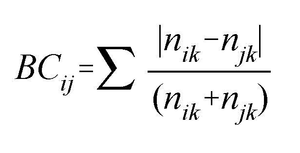
This index compares
the relative proportion of each element in each sample by
subtracting one from the other. The values for all the elements
are summed and subtracted from one. Two samples are considered
to be identical if they have a proportional similarity of
1 and completely dissimilar with a value of 0. During the
process of "classification," each sample was compared
with all other samples and all possible groups of samples.
Finally a representation of which samples are most similar
to each other is determined. The samples then are arranged
in series of groups based on relative similarity. The graphical
representations of such relative similarity lineages resulting
from these analyses are called dendrograms (see Figures 1-4).
Such dendrograms typically show clusters of samples, and hence
the whole process of classification is sometimes called "cluster
analysis." Such an analysis results in an unambiguous,
quantitative and replicable way of showing sample similarity.
Subsequent to the
classification were examined by ordination. Ordination is
a statistical approach and methodology used to suggest interrelationships
between samples. There are a number of different techniques
to do this, I used the process called Principal Coordinate
Analysis as it has fewer inherent biases than many of the
other processes, provided the data are appropriate and the
process is done correctly.
In our natural
three-dimensional world, objects may be described and compared
based on the three principal dimensional axes of length, width,
and height. Ordination results in a similar comparison, but
in an artificial universe with more than three dimensions.
In the case of this study, ordination may be thought of as
a process of creating a mathematically defined universe and
arraying the samples in it based on their relative chemical
concentrations. This universe would not have just the normal
three spatial dimensions. Instead, it would have a number
of dimensions corresponding to the total number of chemicals
or constituents being tested. The data from the samples are
placed in the volume created in this universe and manipulated
to "explain" most of the differences between them
by creating and rotating the dimensional axes to maximize
the differences on the first axis, while minimizing those
differences on all subsequent ones. Ideally, one tries construct
these axes so that most of the information is contained on
the first three axes.
Most people, including
me, have significant trouble visualizing a fourth, fifth,
sixth or seventh dimensional volume (or in the case of this
study, a 30 to 40 dimensional volume). Three dimensions work
just fine, for visualizations, IF we can get there in the
analyses. In diverse data sets such as these, often the sample
variability is so high that one really does need to think
about the samples in five or more dimensions. In these cases,
we are generally out of luck as far as visualizing the samples,
and have to deal with paper data. For these ordination analyses,
the data were classified using Gower's Distance Index, and
the concentrations were zero mean and unit variance transformed.
Subsequent
to Ordination, the centroid of the data in the volume determined
by first three primary axes in ordination space was calculated
and a non-parametric (Mann-Whitney) 95% Confidence Interval
Interval was calculated about that centroid (See Bloom, 1994,
for this procedure and for a good description of classification
and ordination techniques).
To help interpret
the data, particularly the classification and ordination the
sample ranks for each constituent were calculated. The top
three and the bottom three ranks were generally determined.
Results
A summary of the
concentration data is given in Table 1. Although some chemicals,
particularly Calcium and Sodium, are generally found in values
that approximate those of natural seawater, the data are more
notable for the diversity of values than for their consistency.
Many of the rarer trace elements, such as Beryllium and Selenium,
if present, were below detectable levels. Generally, toxic
materials such as Cadmium, Lead and Mercury were also undetectable.
In contrast, the
values for other materials, notably Antimony, Cobalt, and
Titanium were hundreds of times more concentrated in the average
sample than in natural seawater.
|
Table
1. Summary of Concentration Data. Results of 23
samples. Concentrations in µg/l (– ppm). The mean value is the arithmetic
average of the values, SSTD = sample standard deviation.
IO = Instant Ocean , N = number of samples having
the chemical, NSW = Natural Sea Water, T= trace value,
less than 0.0001µg/l in sea water. In the columns where
the Mean Value is given as a Proportion of NSW and IO,
a value of 1.00 would mean that the chemical in question
was equal to the compared value. For example, Calcium
has a value of 1.00 in the columns for both NSW and
IO, and the Mean Value was, therefore, the same as the
value in both NSW and IO.
|
|
|
Concentration
|
Mean Value as a Proportion of
|
IO
|
|
|
Sea
|
|
Sample
|
|
|
|
A.Chemical
|
Water
|
T
|
Mean
± SSTD
|
Max
|
Min
|
N
|
Range
|
NSW
|
IO
|
|
|
Aluminum
|
1.900
|
|
0.173
± 0.070
|
0.320
|
0.070
|
22
|
0.250
|
0.09
|
1.57
|
0.110
|
|
Antimony
|
0.000
|
t
|
0.018
± 0.007
|
0.030
|
0.010
|
12
|
0.020
|
1833
|
0.92
|
0.020
|
|
Arsenic
|
0.024
|
|
0.0200
|
0.020
|
0.020
|
1
|
0.000
|
0.83
|
|
|
|
Barium
|
0.050
|
|
0.015
± 0.008
|
0.033
|
0.005
|
23
|
0.028
|
0.30
|
0.14
|
0.110
|
|
Beryllium
|
0.000
|
t
|
All
Samples Below Test Detection Limits
|
|
Boron
|
4.600
|
|
3.935
± 1.422
|
9.700
|
2.100
|
23
|
7.600
|
0.86
|
1.16
|
3.400
|
|
Cadmium
|
0.000
|
t
|
All
Samples Below Test Detection Limits
|
|
Calcium
|
400
|
|
400.4
± 85.1
|
560
|
210
|
23
|
350
|
1.00
|
1.00
|
400
|
|
Chromium
|
0.000
|
t
|
All
Samples Below Test Detection Limits
|
|
Cobalt
|
0.0001
|
|
0.037
± 0.031
|
0.0420
|
0.030
|
23
|
0.039
|
643
|
1.90
|
0.034
|
|
Copper
|
0.09
|
|
0.024
± 0.005
|
0.038
|
0.018
|
23
|
0.020
|
0.27
|
1.36
|
0.018
|
|
Iodide
|
0.050
|
|
0.447
± 0.518
|
2.070
|
0.100
|
14
|
1.970
|
8.94
|
1.66
|
0.270
|
|
Iron
|
0.02
|
|
All
Samples Below Test Detection Limits
|
|
Lead
|
0.005
|
|
All
Samples Below Test Detection Limits
|
|
Lithium
|
0.100
|
|
0.666
± 1.462
|
7.100
|
0.015
|
23
|
7.0850
|
6.66
|
2.77
|
0.240
|
|
Magnesium
|
1272
|
|
1326.1
± 138.9
|
1500
|
1000
|
23
|
500
|
1.04
|
0.95
|
1400
|
|
Manganese
|
0.010
|
|
All
Samples Below Test Detection Limits
|
|
Mercury
|
0.0003
|
|
All
Samples Below Test Detection Limits
|
|
Molybdenum
|
0.002
|
|
0.019
± 0.018
|
0.074
|
0.005
|
20
|
0.069
|
9.32
|
3.73
|
0.005
|
|
Nickel
|
0.0005
|
|
0.024
± 0.006
|
0.039
|
0.016
|
23
|
0.023
|
48.00
|
1.20
|
0.020
|
|
Phosphorus
|
0.012
|
|
0.328
± 0.745
|
3.500
|
0.020
|
23
|
3.480
|
27.35
|
6.57
|
0.050
|
|
Potassium
|
380
|
|
405.2
± 61.1
|
600
|
300
|
23
|
300
|
1.07
|
1.10
|
370
|
|
Selenium
|
0.004
|
|
All
Samples Below Test Detection Limits
|
|
Silicon
|
4.000
|
|
1.271
± 1.304
|
2.900
|
0.050
|
21
|
2.850
|
0.32
|
0.85
|
1.500
|
|
Silver
|
0.0003
|
|
All
Samples Below Test Detection Limits
|
|
Sodium
|
10561
|
|
10850
± 1246
|
14000
|
8200
|
23
|
5800
|
1.03
|
1.09
|
10000
|
|
Strontium
|
13
|
|
6.783
± 1.694
|
10.000
|
4.100
|
23
|
5.900
|
0.52
|
0.45
|
15
|
|
Sulfur
|
884
|
|
789.6
± 68.9
|
920
|
650
|
23
|
270
|
0.89
|
1.10
|
720
|
|
Thallium
|
0.0005
|
|
0.015
± 0.005
|
0.020
|
0.010
|
15
|
0.010
|
30.66
|
|
|
|
Tin
|
0.003
|
|
0.095
± 0.009
|
0.110
|
0.076
|
23
|
0.034
|
31.77
|
1.11
|
0.086
|
|
Titanium
|
0.0000
|
t
|
0.007
± 0.001
|
0.009
|
0.005
|
22
|
0.004
|
705
|
0.78
|
0.009
|
|
Vanadium
|
0.0003
|
|
0.023
± 0.047
|
0.037
|
0.030
|
23
|
0.007
|
138
|
2.43
|
0.017
|
|
Yttrium
|
0.0003
|
|
All
Samples Below Test Detection Limits
|
|
Zinc
|
0.014
|
|
0.212
± 0.021
|
0.260
|
0.190
|
23
|
0.070
|
15.12
|
1.01
|
0.210
|
| B.
Nitrogen Compounds and Conventional Nutrients |
|
Ammonia
|
|
|
0.036
± 0.017
|
0.092
|
0.030
|
21
|
0.062
|
|
2.44
|
0.024
|
|
Total
Nitrogen
|
|
|
0.619
± 0.313
|
1.300
|
0.030
|
23
|
1.270
|
|
17.62
|
0.052
|
|
Nitrate+Nitrite
|
|
|
11.19
± 18.39
|
62.00
|
0.012
|
20
|
61.99
|
|
28
|
0.400
|
|
Ash
|
|
|
87.26
± 2.05
|
91.00
|
85.000
|
23
|
6.000
|
|
0.97
|
90.00
|
|
Calories
|
|
|
0.00
± 0.00
|
0.00
|
0.00
|
23
|
0.00
|
|
|
|
|
Carbohydrates
|
|
|
0.00
± 0.00
|
0.00
|
0.00
|
23
|
0.00
|
|
|
|
|
Fat
|
|
|
1.361
± 0.940
|
3.20
|
0.00
|
23
|
3.20
|
|
|
|
|
Moisture
|
|
|
96.1
± 0.3
|
97.00
|
96.00
|
23
|
1.00
|
|
1.00
|
96.0
|
|
Total
Protein
|
|
|
0.00
± 0.0
|
0.00
|
0.00
|
23
|
0.00
|
|
|
|
|
C.
System Specifics
|
|
Volume
(U.S. gallons)
|
|
157
± 99
|
380
|
36
|
|
344
|
|
|
|
|
Age
(years)
|
|
2.06
± 2.57
|
10.00
|
0.15
|
|
9.85
|
|
|
|
|
Sp.
G.
|
|
1.0257
± 0.0006
|
1.0260
|
1.0250
|
|
0.0010
|
|
|
|
In the examination
of similarity differences calculated with the methods used
here, it is often useful to be able to compare the ranking
of various chemicals across the samples. In other words, "Were
there samples that contained consistently high values of many
chemicals (or showed high rankings for those chemicals)? "
Similarly, "Were there samples that were always low?"
The rankings are shown in Table 2, and several samples are
evident for their differences.
As might be expected
from independent samples, the data are clearly scattered.
For example, sample CC is full of extremes; it has high values
of Calcium, Cobalt, Copper, Potassium, Nickel and Phosphorus
and low values of Aluminum, Antimony, Arsenic, Boron, Barium,
Lithium and several other chemicals. Sample S1, on the other
hand is has 12 high ranks and only 1 low rank, while Sample
AH is almost the reverse with 10 low ranks and 1 high rank.
As might be expected there are also a lot of values in between.
In subsequent articles, I will investigate some of causes
and concerns of this disparity in samples.
|
Table
2. Chemical Abundance Ranks Within Each Sample.
The uppermost and lowermost ranks are shown. The highest
rank is number 1; within each chemical the ranks could
range from 1 to 24 or ND (Non-Detectable). To interpret
the ranking work within each chemical, for example,
for the Aluminum sample WW had the highest concentration,
Eb was next. Samples CC, GD, RC1 and RS were tied with
the third lowest. The second lowest was sample SM, and
lowest was sample RC2, which had non-detectable values.
|
|
Rank Values
|
1 or 2
=
|
|
3 or 4
=
|
|
21or 22
=
|
|
23 or 24
=
|
|
ND =
|
|
|
|
|
|
|
Sample
|
IO
|
AC
|
AH
|
CC
|
DC
|
DL
|
EB
|
GD
|
JD1
|
JD2
|
JP
|
MB
|
MM
|
RC1
|
RC2
|
RS
|
S1
|
S2
|
S3
|
SC
|
SM
|
SN
|
SS
|
WW
|
|
Aluminum
|
|
|
|
|
|
|
|
|
|
|
|
|
|
|
|
|
|
|
|
|
|
|
|
|
|
Antimony
|
|
|
|
|
|
|
|
|
|
|
|
|
|
|
|
|
|
|
|
|
|
|
|
|
|
Arsenic
|
|
|
|
|
|
|
|
|
|
|
|
|
|
|
|
|
|
|
|
|
|
|
|
|
|
Boron
|
|
|
|
|
|
|
|
|
|
|
|
|
|
|
|
|
|
|
|
|
|
|
|
|
|
Barium
|
|
|
|
|
|
|
|
|
|
|
|
|
|
|
|
|
|
|
|
|
|
|
|
|
|
Calcium
|
|
|
|
|
|
|
|
|
|
|
|
|
|
|
|
|
|
|
|
|
|
|
|
|
|
Cobalt
|
|
|
|
|
|
|
|
|
|
|
|
|
|
|
|
|
|
|
|
|
|
|
|
|
|
Copper
|
|
|
|
|
|
|
|
|
|
|
|
|
|
|
|
|
|
|
|
|
|
|
|
|
|
Potassium
|
|
|
|
|
|
|
|
|
|
|
|
|
|
|
|
|
|
|
|
|
|
|
|
|
|
Lithium
|
|
|
|
|
|
|
|
|
|
|
|
|
|
|
|
|
|
|
|
|
|
|
|
|
|
Magnesium
|
|
|
|
|
|
|
|
|
|
|
|
|
|
|
|
|
|
|
|
|
|
|
|
|
|
Molybdenum
|
|
|
|
|
|
|
|
|
|
|
|
|
|
|
|
|
|
|
|
|
|
|
|
|
|
Sodium
|
|
|
|
|
|
|
|
|
|
|
|
|
|
|
|
|
|
|
|
|
|
|
|
|
|
Nickel
|
|
|
|
|
|
|
|
|
|
|
|
|
|
|
|
|
|
|
|
|
|
|
|
|
|
Phosphorus
|
|
|
|
|
|
|
|
|
|
|
|
|
|
|
|
|
|
|
|
|
|
|
|
|
|
Sulfur
|
|
|
|
|
|
|
|
|
|
|
|
|
|
|
|
|
|
|
|
|
|
|
|
|
|
Silicon
|
|
|
|
|
|
|
|
|
|
|
|
|
|
|
|
|
|
|
|
|
|
|
|
|
|
Tin
|
|
|
|
|
|
|
|
|
|
|
|
|
|
|
|
|
|
|
|
|
|
|
|
|
|
Strontium
|
|
|
|
|
|
|
|
|
|
|
|
|
|
|
|
|
|
|
|
|
|
|
|
|
|
Titanium
|
|
|
|
|
|
|
|
|
|
|
|
|
|
|
|
|
|
|
|
|
|
|
|
|
|
Thallium
|
|
|
|
|
|
|
|
|
|
|
|
|
|
|
|
|
|
|
|
|
|
|
|
|
|
Vanadium
|
|
|
|
|
|
|
|
|
|
|
|
|
|
|
|
|
|
|
|
|
|
|
|
|
|
Zinc
|
|
|
|
|
|
|
|
|
|
|
|
|
|
|
|
|
|
|
|
|
|
|
|
|
|
Iodide
|
|
|
|
|
|
|
|
|
|
|
|
|
|
|
|
|
|
|
|
|
|
|
|
|
|
Ammonia
|
|
|
|
|
|
|
|
|
|
|
|
|
|
|
|
|
|
|
|
|
|
|
|
|
|
Total
Nitrogen
|
|
|
|
|
|
|
|
|
|
|
|
|
|
|
|
|
|
|
|
|
|
|
|
|
|
Nitrate+Nitrite
|
|
|
|
|
|
|
|
|
|
|
|
|
|
|
|
|
|
|
|
|
|
|
|
|
|
Ash
|
|
|
|
|
|
|
|
|
|
|
|
|
|
|
|
|
|
|
|
|
|
|
|
|
|
Fat
|
|
|
|
|
|
|
|
|
|
|
|
|
|
|
|
|
|
|
|
|
|
|
|
|
|
Moisture
|
|
|
|
|
|
|
|
|
|
|
|
|
|
|
|
|
|
|
|
|
|
|
|
|
|
Sample
Data
|
|
High
Ranks
|
3
|
0
|
1
|
8
|
1
|
3
|
5
|
10
|
1
|
1
|
0
|
2
|
1
|
1
|
4
|
0
|
12
|
5
|
4
|
0
|
0
|
0
|
1
|
3
|
|
Low
Ranks
|
7
|
5
|
10
|
10
|
5
|
5
|
4
|
2
|
3
|
5
|
2
|
2
|
9
|
8
|
7
|
7
|
1
|
1
|
2
|
9
|
6
|
4
|
7
|
6
|
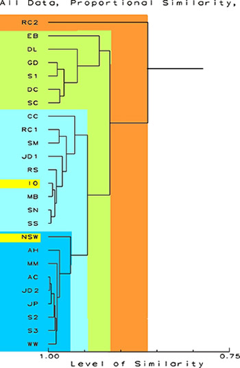
Dendrograms
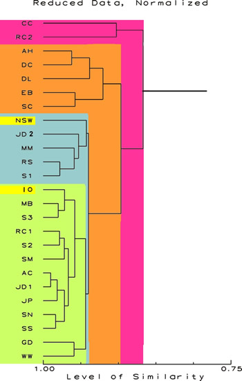
I would imagine
the first thing the average reef aquarist would say when looking
at the figures below is, "Yikes." (Actually, I am
being "polite," I think the first thing said would
be considerably more "earthy and heartfelt.")
Don't despair,
these figures are actually very simple to understand. A dendrogram
is a figure that branches like a tree ("dendron"
means "tree"). In these figures, the trunk is coming
from the left and the branches show relationships, based on
chemical abundances. What they show are the relationships
of the samples indicated at the left. Each branch typically
separates two groups of samples on the basis of shared characters.
Each group has more in common with other members of its group
(and sometimes the group is only the one sample) than all
other samples. So in the first example below, the first branch
point from the right is at a similarity of about 0.86 or 86
percent. That branching splits off sample RC2 from all the
others. All the other samples are more similar to themselves
than to RC2. The second branch occurs at a similarity of about
0.92, and splits the remaining 24 samples into two groups.
The smaller group, consisting of samples EB, DL, GD, S1, DC,
and SC is separated from all other samples. From Table 2,
it is evident that these samples have little overall in common
except that they generally have several extreme ranks of various
chemicals. The larger group is further subdivided into two
other groups of samples each more similar amongst themselves
than to others. Any of the samples in the two shades of blue
are more similar to each other than any of them are to those
samples in green or orange. From examining these data, one
can see that the samples in blue are more similar to either
artificial sea water or natural sea than are the samples in
green or orange. In the discussion session that follows, I
will discuss some of the reasons for these groupings.
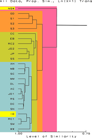
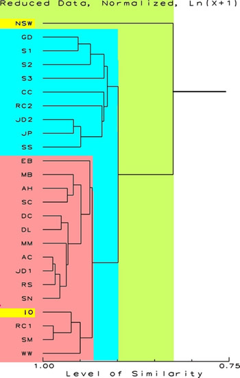
Notice the changes
when all of the data are log normally transformed in Figure
2. Here the effects of very high concentrations are reduced,
and the effects of very small concentrations of chemicals
are enhanced. Natural Sea Water, with a lot of elements in
trace amounts becomes very distinct. All of the other samples
are more than 90 % similar, and even though they are grouped,
these groups are fairly similar amongst themselves. The large
group indicated in gray containing IO is comprised of many
samples that were initially formed from IO water.
Figure 3 shows
the relationships of the samples when the effects of trace
elements present in natural sea water, but below the detection
limits in all the samples, are removed from the analysis.
Most of these samples are actually quite similar to each other
and to NSW and IO. Only a few samples are somewhat oddballs.
Interestingly, these are some of the same dissimilar samples
shown in the upper branches of the dendrogram in Figure 1.
In Figure 4, the
data used in the analysis are log normally transformed, and
as a result, NSW is again separated from all other samples.
This is undoubtedly due to the abundance of elements present
in trace amounts. Such materials really don’t exist in
the aquarium samples; the samples either have materials in
relatively great amounts, or they lack them all together.
All of the remaining samples are at least 90% similar, and
include IO. No matter what has been done to these aquaria,
the water in them is still very similar across all the samples.
 |
|
Figure
1.
Proportional Similarity Index Dendrogram showing the
relative similarity of the sample. The scale at the
bottom is in percent similarity. All data are included
and no transformations have been done. The data for
NSW and IO are highlighted.
|
 |
|
Figure
2.
Proportional Similarity Index Dendrogram showing the
relative similarity of the sample. The scale at the
bottom is in percent similarity. All data are included
and the ln (x+1) transformations have been done. This
emphasizes the contribution of rarer chemicals. The
data for NSW and IO are highlighted.
|
 |
|
Figure
3.
Proportional Similarity Index Dendrogram showing the
relative similarity of the sample. The scale at the
bottom is in percent similarity. This figure shows the
relationships with the values for sodium and undetectable
elements removed. No ln (x+1) transformations have been
done. This de-emphasizes the contribution of rarer chemicals
and sodium in the NSW data. The data for NSW and IO
are highlighted.
|
 |
|
Figure
4.
Proportional Similarity Index Dendrogram showing the
relative similarity of the sample. The scale at the
bottom is in percent similarity. This figure shows the
relationships with the values for sodium and undetectable
elements removed, and the ln (x+1) transformations have
been done. This further de-emphasizes the contribution
of rarer chemicals and sodium in the NSW data. The data
for NSW and IO are highlighted.
|
|
Table
3.
Ordination results using the reduced data set (sodium,
and chemicals below the detection limits in all the
test samples removed). The data were normalized by multiplication
(sample Sodium concentration/NSW Sodium concentration). There
were 25 samples (23 test samples, 1 IO sample, and the
data for NSW) and 28 chemical attributes were considered. The
samples were standardized to a zero mean, with a unit
variance. The index of classification was Gowers distance
measure.
|
|
A.
Efficiency of the dimension at explaining the variation
between the samples
|
|
Dimension
(Vector)
|
Efficiency
|
Cumulative
Variance Explained
|
|
1
|
58.24
|
58.24
|
|
2
|
24.58
|
82.82
|
|
3
|
13.58
|
96.40
|
|
4
|
1.98
|
98.38
|
|
5
|
1.41
|
99.79
|
|
6-25
|
0.21
|
100.00
|
The
numerical results of the efficiency of the ordination at grouping
the data in similar groups (or in the language of the test
"explaining the variation") are indicated in Table
3. It can be seen that manipulations along the first 3 dimensions
(or vectors) explain over 96 percent of the variation. This
is really a quite good result. Normally, one considers that
an ordination result is good if this value is 75 percent or
better. This means we can use the data derived from the ordinations,
with some degree of confidence.
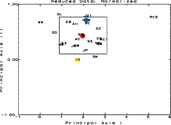
The following illustrations,
Figures 5-7, are perhaps the most important figures in the
article. They show the result of the ordination analyses in
a three-dimensional space with each axis corresponding to
the dimensions indicated above; each figure shows the plot
of the data from a different direction. The positions for
the centroid of the sample grouping, IO and NSW are indicated.
The rectangle in the center each figure is the representation
of the 95% Confidence Interval Limits around the centroid.
That means that one can say that any sample outside of the
boundary of that line is statistically significantly different
from centroid of the group, with a 95% chance that that statement
is correct. Or phrased another way, all of the samples shown
as being outside the line in any one of the views have only
one chance in twenty - or less - of being similar to the samples
inside the limits.
This technique
and the dendrograms do show that there are some defined groups
of samples that have within themselves similar samples. There
are also a large number of samples, including specifically
both NSW and IO, that have chemical constituent arrays that
are statistically significantly different from the majority
of the samples.
The take home message
from these results is that there are some discrete groups
of samples, but that at least a third of the samples are from
aquaria that vary in some significant way not only from each
other, but from both natural sea water, and artificial sea
water made from one of the most popular of artificial sea
water mixes.
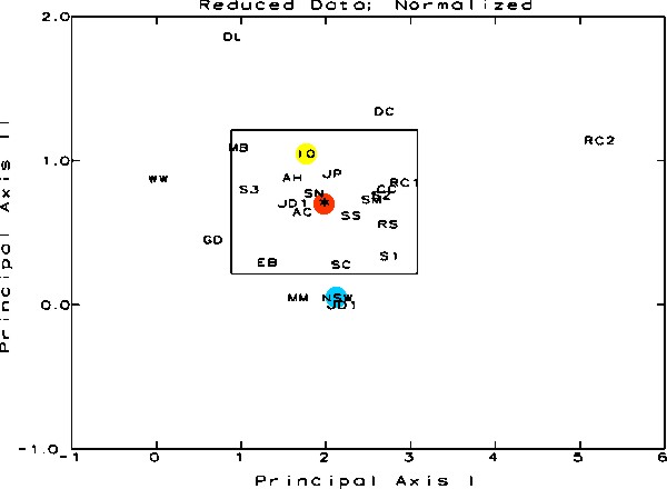
Figure
5.
This figure is a result of the Principal Coordinate and Recovery
Analysis. The samples are represented by their letter designations
and should be visualized in 3-Dimensional space. The three
axes for this space are Principal Axes I, II, and III, each
oriented perpendicular to one other. This figure shows the
data in relation to Principal Axes I and II. The rectangle
is the 95% Confidence Interval around the centroid of the
distribution. Any sample shown outside the limits in any one
graph is statistically significantly different from the average
of all of the samples. The position of the cluster centroid
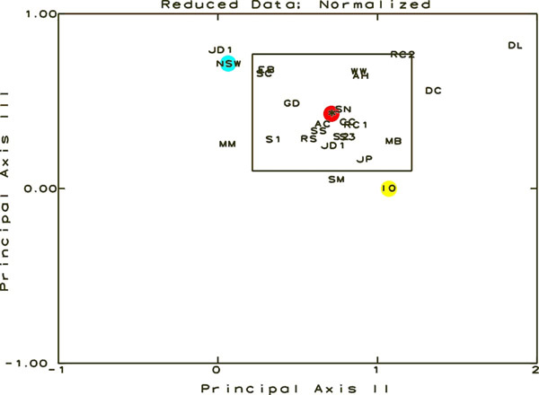
is shown in red, NSW in blue and IO in yellow. |
|
Figure
6.
This figure is a result of the Principal Coordinate
and Recovery Analysis. The samples are represented by
their letter designations and should be visualized in
3-Dimensional space. The three axes for this space are
Principal Axes I, II, and III, each oriented perpendicular
to one other. This figure shows the data in relation
to Principal Axes I and III. The rectangle is the 95%
Confidence Interval around the centroid of the distribution.
Any sample shown outside the limits in any one graph
is statistically significantly different from the average
of all of the samples. The position of the cluster centroid
is shown in red, NSW in blue and IO in yellow.
|
|
Figure
7.
This figure is a result of the Principal Coordinate
and Recovery Analysis. The samples are represented by
their letter designations and should be visualized in
3-Dimensional space. The three axes for this space are
Principal Axes I, II, and III, each oriented perpendicular
to one other. This figure shows the data in relation
to Principal Axes II and III. The rectangle is the 95%
Confidence Interval around the centroid of the distribution.
Any sample shown outside the limits in any one graph
is statistically significantly different from the average
of all of the samples. The position of the cluster centroid
is shown in red, NSW in blue and IO in yellow.
|
|
Table
4. Maximum and Minimum Values from the Study as
Proportion of the Same Element in Natural Sea Water.
The proportional concentrations were calculated by dividing
the test maximum and minimum values by the NSW concentrations.
|
|
|
Proportional Concentrations
|
Actual Concentrations
|
|
Chemical
|
Symbol
|
Maximum
|
Minimum
|
Sea Water
|
|
Aluminum
|
Al
|
0.1684
|
0.0368
|
1.9000
|
|
Antimony
|
An
|
3000.
|
1000.
|
Trace, Less than
0.0001 µg/l
|
|
Arsenic
|
As
|
0.8333
|
0.8333
|
0.0240
|
|
Boron
|
B
|
2.1087
|
0.4565
|
4.6000
|
|
Barium
|
Ba
|
0.6600
|
0.1000
|
0.0500
|
|
Beryllium
|
Be
|
Not Detected.
|
0.0001
|
|
Calcium
|
Ca
|
1.4000
|
0.5250
|
400.
|
|
Cadmium
|
Cd
|
Not Detected.
|
Trace, Less than
0.0001 µg/l
|
|
Cobalt
|
Co
|
420.
|
300.
|
0.0001
|
|
Chromium
|
Cr
|
Not Detected.
|
Trace, Less than
0.0001 µg/l
|
|
Copper
|
Cu
|
0.4222
|
0.2000
|
0.0900
|
|
Iron
|
Fe
|
Not Detected.
|
0.0200
|
|
Mercury
|
Hg
|
Not Detected.
|
0.0003
|
|
Potassium
|
K
|
1.5789
|
0.7895
|
380.
|
|
Lithium
|
Li
|
71.00
|
0.15
|
0.1000
|
|
Magnesium
|
Mg
|
1.1792
|
0.7862
|
1272.
|
|
Manganese
|
Mn
|
Not Detected.
|
0.0100
|
|
Molybdenum
|
Mo
|
37.00
|
2.5000
|
0.0020
|
|
Sodium
|
Na
|
1.3256
|
0.7764
|
10561.
|
|
Nickel
|
Ni
|
78.00
|
32.
|
0.0005
|
|
Phosphorus
|
P
|
291.6667
|
1.6667
|
0.0120
|
|
Lead
|
Pb
|
Not Detected.
|
0.0050
|
|
Sulfur
|
S
|
1.0407
|
0.7353
|
884.
|
|
Selenium
|
Se
|
Not Detected.
|
0.0040
|
|
Silicon
|
Si
|
0.7250
|
0.0125
|
4.
|
|
Silver
|
Ag
|
Not Detected.
|
0.0003
|
|
Tin
|
Sn
|
36.6667
|
25.3333
|
0.0030
|
|
Strontium
|
Sr
|
0.7692
|
0.3154
|
13.
|
|
Titanium
|
Ti
|
900.
|
500.
|
Trace, Less than
0.0001 µg/l
|
|
Thallium
|
Tl
|
40.
|
20.
|
0.0005
|
|
Vanadium
|
V
|
123.3333
|
100.
|
0.0003
|
|
Yttrium
|
Y
|
Not Detected.
|
0.0003
|
|
Zinc
|
Zn
|
18.5714
|
13.5714
|
0.0140
|
|
Iodide
|
I
|
41.4000
|
2.
|
0.0500
|
|
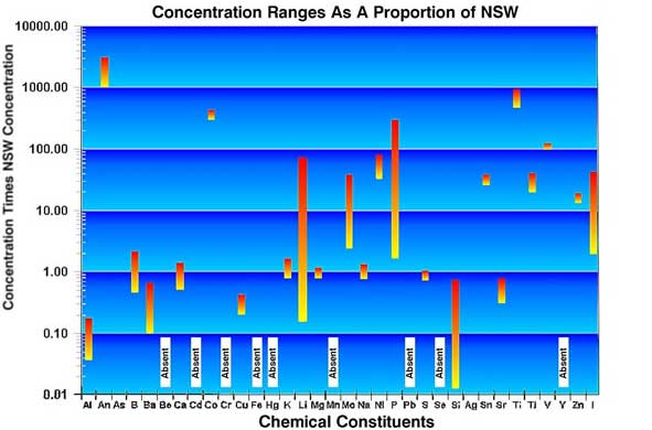
Figure
8.
This figure is a graphical representation of the data
in Table 3. Note that the concentration ranges are given
on a logarithmic scale. Values near 1.00 are similar
to NSW, those greater or lesser are proportionally different
from NSW.
|
Discussion
and Conclusions
Many hobbyists are fond of saying that
there is no "one" correct way to set up a reef tank,
that instead of "One True Path Toward Righteousness and
Light," there are an almost infinite number of ways to
set up a reef tank. Well, even the most adventurous of these
folks would likely not have guessed the differences found
in these 23 reef tanks, some with problems (more about that
in subsequent articles), but even so, all are supporting a
broad and diverse array of animals.
In most cases, it appears that about the
only similarities that Reef Aquarium Water has to Natural
Sea Water is that they both are wet, and they both contain
somewhere in the range of three and one half percent (or 35%)
salt by weight. It can truly be said that very little else
is similar. The proportional data given in Table 4 and Figure
8 show that while some of the constituents in these tanks
are near the proportions found in sea water, some others are
absent, for example Beryllium; a few are present in very reduced
proportions, for example Aluminum; and others are present
in significantly higher proportions, such as Antimony, Titanium,
and Iodide. While many of the chemicals are found in similar
amounts in all the tanks, others vary widely. Lithium, for
example, varies between the largest and smallest concentrations
by almost a factor of 500 times.
Nevertheless, the tank waters surveyed
in this study are apparently relatively similar in many regards.
The dendrograms generally show that while there are a group
of "outlier" samples, most of the samples are clustered
in one to four groups all similar to each other with about
Proportional Similarities from about 85 percent to 90 percent.
This similarity is likely due to the widespread usage of Instant
Ocean™ as the salt mix used by the aquarists in the study.
However, interestingly enough, many of these same tanks are
in different similarity clusters from that containing Instant
Ocean™.
Even though many of the systems start at
the same point, and have some overall similarities, the cumulative
results of the factor-by-factor differences, indicate that
the overall sample group is statistically significantly different
from both IO and NSW. This is indicated in Figures 5-7, where
it is evident that the artificial and natural sea waters have
distributions that are statistically significantly different
from the average point (the sample "centroid") describing
all the samples.
Most aquarists aspire to the goal of maintaining
the liquid medium in their aquarium as similar to NSW as is
possible. Yet, they try to do this without any way to test
most chemicals, and without an understanding of the dynamic
nature of the concentration of those chemicals in semi-closed
systems such as these aquaria. A significant reason for this
problem is that the basic water obtained when artificial salt
mixes (see Atkinson and Bingman, 1999 and the IO data in this
study) are prepared bears very little similarity to NSW, but
even aquarists using NSW as the initial medium don't have
tanks where the chemical composition bears much similarity
to Natural Sea Water. Sample GD was from a tank that uses
NSW as a medium, and as shown in the dendrograms, no matter
how the data are manipulated, that particular sample is never
very similar to NSW.
Questions as to why these differences occur,
and discussions of their importance will be the subject of
the subsequent articles discussing the results of this project.
For the present, it is apparent that much of the worry over
various chemical compositions and levels is simply unnecessary.
It appears that the animals have significant latitude in altering
either their external or internal environments to adjust for
the differences seen in this study.
|